Electrostatic Potential with Spherical Boundary Conditions

One of the many mathematical techniques that are useful in the study of electrostatics is called the separation of variables method. This topic covers the application of this method to a situation in which the electrostatic potential in a spherically symmetric system is known. In such a system, the potential (potential and electrostatic potential are interchangeable here) everywhere in space is a function described by the Legendre polynomials. To remind yourself of why this is so, review treatments of Laplace’s equation in spherical coordinates. The following discussion takes the form of the potential as the starting point and then demonstrates a way to use this method for determining more about the system.

Consider a grounded sphere of radius a that is made of a conducting material. This conducting, and solid, sphere is then covered by a shell made of an insulating material. The insulation material is a shell with radius b, in which it is required that b > a (treat the shell as though it has no thickness). The electrostatic potential on the insulating shell, Φ_shell, is known to be,

$\phi_\text{shell} = \alpha \sin^2(\theta)$

where α is a constant and θ is the angular coordinate of the spherical coordinate system. Figure 1 shows the setup for this topic.

For this system we will find the electrostatic potential everywhere in space and then determine the charge densities on the spherical objects.

Figure 1: Setup for this topic. The central, solid, sphere is grounded to achieve a potential of zero. The enclosing shell potential is also shown. While not shown in this figure, the potential at r = infinity is also zero, this time by definition.

Spatial Profile of Scalar Potential

To begin, the only charge densities we can possibly solve for are surface charge densities. The enclosing shell is just that, a shell, and therefore has no inner volume in which charge may be found. This is just part of the definition for this setup, so there is no physical intuition to be gained. The solid sphere is a conductor and any charge density within it will reside on the surface. This is part of the definition of conductors and is a generally applicable piece of electrodynamic theory. The volume charge density inside of the solid sphere is zero, though it remains to solve for the charge density on the surface of this sphere (i.e., at r = a).

It is possible to solve for the charge densities after we have determined the value of the potential everywhere in space. For this spherically symmetric system the form of the potential is given by a sum over Legendre polynomials. The potential of the solid sphere is given, as is the potential at infinity, so the potential is described by,

$\phi = 0 \quad \text{for} \quad r \le a$
$\phi = 0 \quad \text{for} \quad r \rightarrow \infty$

and it remains to solve for the regions between the objects and beyond the shell. These expressions serve as two of the three boundary conditions given. The third boundary condition is given by the potential on the shell.

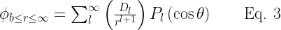
Between the objects, for a ≤ r ≤ b, the solution for the potential is given by the complete sum over Legendre polynomials,

$\phi_{a\le r \le b} = \sum^\infty_l \left(A_lr^l+ \frac{B_l}{r^{l+1}} \right) P_l\left(\cos\theta \right) \quad\quad\text{Eq. 1}$

where P_l(cosθ) represents the l^th Legendre polynomial with cosθ as its argument and A, B are constants. The actual Legendre functions will be written out every time they need to be for further algebraic progress. Again, this expression represents the total solution for this region. This is the starting point for solving any similar (i.e., electrostatic potential) problem in spherical coordinates.

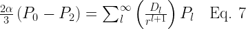
The functional form of the potential for the region b ≤ r ≤ ∞ begins with the expression in Eq. 1.

$\phi_{b\le r \le \infty} = \sum^\infty_l \left(C_lr^l+ \frac{D_l}{r^{l+1}} \right) P_l\left(\cos\theta \right) \quad\quad\text{Eq. 2}$

where C, D are the same type of constants as A, B, but not equal to them. In this case the potential must go to zero as r → ∞, therefore all of the constants, C_l, must be zero. The form of the potential in this region simplifies to,

$\phi_{b\le r \le \infty} = \sum^\infty_l \left(\frac{D_l}{r^{l+1}} \right) P_l\left(\cos\theta \right)\quad\quad\text{Eq. 3}$

where all that remains is to perform some algebra to rewrite these with the numerical values of the A, B, and D constants. The phrase “some algebra” usually means a significant amount of tedious labor is on its way, as is the case here.

Beginning with Eq. 3, we know the exact value this expression must equal at the position r = b. This is given in the setup,

$\phi_{r = b} = \alpha\sin^2(\theta) = \sum^\infty_l \left(\frac{D_l}{r^{l+1}} \right) P_l\left(\cos\theta \right)\quad\quad\text{Eq. 4}$

and it seems difficult to equate these in a manner that allows for the determination of the infinite values of D. It is reasonable to assume that there are not an infinite number of D‘s for which a value must be found. Rewriting the α sin²θ term as a function of Legendre polynomials will help simplify matters. Since our Legendre polynomials take the cosθ as an argument it is a good idea to begin with the equality sin²θ = 1 – cos²θ and then take the simplest Legendre polynomial that includes the cos²θ term (after the first line I am going to start using shorthand P_l = P_l(cosθ)),

$P_2\left(\cos\theta \right) = \frac{1}{2} \left( 3\cos^2\theta - 1\right)$
$2P_2 =3\cos^2\theta - 1$
$\frac{1}{3}\left(2P_2 + 1\right) = \cos^2\theta \quad\quad\text{Eq. 5}$

and now we can rewrite,

$\alpha\sin^2\theta = \alpha \left(1 - \cos^2\theta \right)$
$\alpha\sin^2\theta = \alpha \left[1 - \frac{1}{3}\left(2P_2 +1 \right) \right]$
$\alpha\sin^2\theta = \alpha \left[ 1 - \frac{2}{3}P_2 - \frac{1}{3}\right]$
$\alpha\sin^2\theta = \alpha \left(\frac{2}{3} - \frac{2}{3}P_2 \right)$
$\alpha\sin^2\theta = \frac{2\alpha}{3}\left(1 - P_2 \right)$
$\alpha\sin^2\theta = \frac{2\alpha}{3}\left(P_0 - P_2 \right)\quad P_0 = 1\quad\text{Eq. 6}$

where we have only needed to employ the expressions for two of the Legendre polynomials.

Combining the results of Eq. 4 and Eq. 6 we have,

$\frac{2\alpha}{3}\left(P_0 - P_2 \right) = \sum^\infty_l\left( \frac{D_l}{r^{l+1}}\right)P_l\quad\text{Eq. 7}$

and the left side shows us that only the l = 0 and l = 2 terms must be kept. Technically, it means that D_l = 0 for every value of l except 0 and 2. The reason for this matching is that the Legendre polynomials are orthogonal.

The non-zero D values are found by writing out the sum in Eq. 7 and equating terms with the same l values,

$\frac{2\alpha}{3}\left(P_0 - P_2 \right) = \frac{D_0}{b}P_0 + \frac{D_2}{b^3}P_2$

$\frac{2\alpha}{3}P_0 = \frac{D_0}{b}P_0 \rightarrow D_0 = \frac{2\alpha b}{3}$

$-\frac{2\alpha}{3}P_2 = \frac{D_2}{b^3}P_2 \rightarrow D_2 = -\frac{2\alpha b^3}{3}$

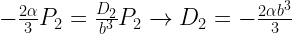
where this provides the solution all the way out to r → ∞ and we may add a piece to our map of the potential.

$\phi = 0 \quad\text{for}\;\; r\le a$

$\phi = \frac{2\alpha b}{3r}P_0 + \frac{-2\alpha b^3}{r^3}P_2 \quad\text{for}\;\; b \le r \le \infty$

where it is seen that as r approaches infinity, the inverse r terms will quickly go to zero.

At the position r = b, the value of Eq. 1 must also be equal to Eq. 6. Equating these gives,

$\phi_{r=b} = \sum^\infty_l \left( A_l r^l + \frac{B_l}{r^{l+1}}\right) P_l\left( \cos\theta\right) = \frac{2\alpha}{3}\left(P_0 - P_2 \right)$

and we are once again in a position to remove all but two values of l.

The previous equality simplifies to,

$\left(A_0b^0 + \frac{B_0}{b} \right)P_0 + \left(A_2b^2 + \frac{B_2}{b^3} \right)P_2 = \frac{2\alpha}{3}\left( P_0 - P_2\right)$

and there are two more equations found by equating similar Legendre polynomial terms.

$\left(A_0 + \frac{B_0}{b} \right)P_0 = \frac{2\alpha}{3}P_0 \quad\quad \quad\left(A_2b^2 + \frac{B_2}{b^3} \right)P_2 = -\frac{2\alpha}{3}P_2$

$A_0 + \frac{B_0}{b} = \frac{2\alpha}{3}\quad\quad \quad A_2b^2 + \frac{B_2}{b^3} = -\frac{2\alpha}{3} \quad\text{Eq. 8}$

and the issue now is that we have four unknowns and only two equations.

Another set of equations containing these unknowns may be achieved by examining the remaining boundary at r = a. The potential is zero here, but still described by Eq. 1. This leads to,

$\left(A_0a^0 + \frac{B_0}{a} \right)P_0 + \left(A_2a^2 + \frac{B_2}{a^3} \right) P_2 = 0$

$A_0 + \frac{B_0}{a} = 0 \quad\quad\quad A_2a^2 + \frac{B_2}{a^3} = 0$

$A_0 = -\frac{B_0}{a} \quad\quad\quad A_2 = -\frac{B_2}{a^5} \quad\text{Eq. 9}$

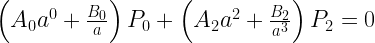
and these are combined with the previous two equations to solve for the a and b constants.

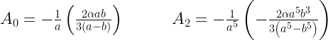
Inserting Eq. 9 into Eq. 8 gives,

$-\frac{B_0}{a} + \frac{B_0}{b} = \frac{2\alpha}{3} \quad\quad\quad -\frac{B_2}{a^5}b^2 + \frac{B_2}{b^3} = -\frac{2\alpha}{3}$

$B_0\left( \frac{1}{b} - \frac{1}{a}\right) = \frac{2\alpha}{3} \quad\quad\quad B_2\left(-\frac{b^2}{a^5} + \frac{1}{b^3} \right) = -\frac{2\alpha}{3}$

$B_0\left( \frac{a-b}{ab} \right) = \frac{2\alpha}{3} \quad\quad\quad B_2\left(\frac{-b^5 + a^5}{a^5b^3} \right) = -\frac{2\alpha}{3}$

$B_0 = \frac{2\alpha ab}{3(a-b)} \quad\quad\quad B_2 = -\frac{2\alpha a^5b^3}{3\left( a^5 - b^5\right)}$

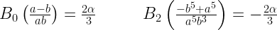
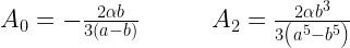
and the corresponding values of the A‘s from Eq. 9 are,

$A_0 = -\frac{1}{a}\left( \frac{2\alpha ab}{3(a-b)}\right)\quad\quad\quad A_2 = -\frac{1}{a^5}\left(-\frac{2\alpha a^5b^3}{3\left( a^5 - b^5\right)} \right)$

$A_0 = - \frac{2\alpha b}{3(a-b)}\quad\quad\quad A_2 = \frac{2\alpha b^3}{3\left( a^5 - b^5\right)}$

With all of these constants known and the form of Eq. 1, the potential may be written,

$\phi = 0 \quad\quad \text{for}\;\;r\le a$

$\phi = \left(A_0 + \frac{B_0}{r} \right)P_0 + \left(A_2r^2 + \frac{B_2}{r^3} \right)P_2 \quad\quad \text{for}\;\;a\le r \le b$

$\phi = \frac{2\alpha b}{3r}P_0 + \frac{-2\alpha b^3}{r^3}P_2 \quad\quad \text{for}\;\;b\le r \le \infty$

where the full expression for the region between the spheres is,

$\phi_{a\le r \le b} = \left(-\frac{2\alpha b}{3(a-b)} + \frac{2\alpha ab}{3r(a-b)} \right)P_0 + \left( \frac{2\alpha b^3r^2}{3\left( a^5 - b^5\right)} + (-1)\frac{2\alpha a^5b^3}{3r^2\left( a^5 - b^5\right)} \right)P_2$

Surface Charge Density

A key expression for determining the surface charge density, σ, at a location for which the electric fields above, E_above, and below, E_below, it are known, is,

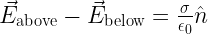
$\vec{E}_\text{above} - \vec{E}_\text{below} = \frac{\sigma}{\epsilon_0}\hat{n}$

where n is the normal vector pointing away from (i.e., above) the surface and ε_o is the permittivity of free space. Since the electric field can be written in terms of the potential as E = –∇Φ, the previous expression may be written as,

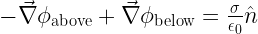
$-\vec{\nabla}\phi_\text{above} + \vec{\nabla}\phi_\text{below} = \frac{\sigma}{\epsilon_0}\hat{n}$

and since we are spherically symmetric there will only be a gradient along the radial direction. This becomes a one dimensional system and a further simplification is available,

$\frac{\partial\phi_\text{below}}{\partial r} - \frac{\partial\phi_\text{above}}{\partial r} = \frac{\sigma}{\epsilon_0}\hat{n}$

As we have already determined that charge density exists at r = a, b, let us now apply the previous equation to determine the value of these densities. For r = a the region below the surface is 0 ≤ r < a (with a potential of zero) and the region above the surface is a < r ≤ b. At this surface the normal vector is directed along the radial direction, n = +r. In the following steps the substitution r = a is made just after the derivative is calculated,

$\frac{\sigma}{\epsilon_0} = \frac{\partial}{\partial r}(0) - \frac{\partial}{\partial r}\left[\left(A_0 + \frac{B_0}{r} \right)P_0 + \left( A_2r^2 + \frac{B_2}{r^3}\right)P_2\right]$

$\frac{\sigma}{\epsilon_0} = -\frac{\partial}{\partial r}(A_0P_0) - \frac{\partial}{\partial r}\left(\frac{B_0}{r}P_0\right) - \frac{\partial}{\partial r}\left(A_2r^2P_2 \right) - \frac{\partial}{\partial r}\left( \frac{B_2}{r^3}P_2\right)$

$\frac{\sigma}{\epsilon_0} = -0 - B_0P_0\left(\frac{-1}{r^2}\right) - A_2P_2(2r) - B_2P_2\left(\frac{-3}{r^4}\right)$

$\frac{\sigma}{\epsilon_0} = \frac{B_0P_0}{a^2} - 2aA_2P_2 + \frac{3B_2P_2}{a^4}$

$\frac{\sigma}{\epsilon_0} = \frac{2\alpha b}{3a(a-b)} - \frac{4\alpha ab^3}{3\left(a^5 - b^5 \right)}P_2 + \left(-\frac{2\alpha ab^3}{a^5-b^5}P_2 \right)$

$\frac{\sigma}{\epsilon_0} = \frac{2\alpha b}{3a(a-b)} - \left[ \frac{4\alpha ab^3}{3\left(a^5 - b^5 \right)} + \frac{6\alpha ab^3}{3\left( a^5 - b^5\right)}\right]P_2$

$\sigma = \epsilon_0 \left( \frac{2\alpha b}{3a(a-b)} - \frac{10\alpha ab^3}{3\left(a^5 - b^5 \right)}P_2\right) \quad\text{Eq. 10}$

where this is the charge density of the surface at r = a and P₂ is given in Eq. 5.

The same procedure is applicable in the pursuit of the charge density on the shell located at r = b. In this case the below region is that between the spheres and the above region is the solution for b ≤ r ≤ ∞. Our work is made easier because the derivative for the below region has been done in Eq. 10, we begin at that step and replace the r‘s with b‘s (also multiply the entire expression by -1 because it was the above region in the previous case) for the present situation.

We have,

$\frac{\sigma_b}{\epsilon_0} = -\frac{B_0P_0}{b^2} + 2bA_2P_2 - \frac{3B_2P_2}{b^4} - \frac{\partial\phi_\text{above}}{\partial r}$

$\frac{\sigma_b}{\epsilon_0} = -\frac{B_0P_0}{b^2} + 2bA_2P_2 - \frac{3B_2P_2}{b^4} - \left[ \frac{\partial}{\partial r}\left( \frac{2\alpha b}{3r}P_0 - \frac{2\alpha b^3}{r^3}P_2\right)\right]$

$\frac{\sigma_b}{\epsilon_0} = -\frac{B_0P_0}{b^2} + 2bA_2P_2 - \frac{3B_2P_2}{b^4} - \left[ \frac{2\alpha b}{3}\left( -\frac{1}{r^2}\right)P_0 - 2\alpha b^3\left(-\frac{3}{r^4} \right)P_2 \right]$

$\frac{\sigma_b}{\epsilon_0} = -\frac{B_0P_0}{b^2} + 2bA_2P_2 - \frac{3B_2P_2}{b^4} + \frac{2\alpha}{3b}P_0 - \frac{6\alpha}{b}P_2$

$\frac{\sigma_b}{\epsilon_0} = -\frac{2\alpha a}{3b(a-b)} + \frac{4\alpha b^4}{3\left(a^5-b^5 \right)}P_2 + \frac{2\alpha a^5}{b\left( a^5 - b^5\right)}P_2 + \frac{2\alpha}{3b} - \frac{6\alpha}{b}P_2$

$\frac{\sigma_b}{\epsilon_0} = -\frac{2\alpha a}{3b(a-b)} + \frac{2\alpha}{3b} + \left[ \frac{4\alpha b^4}{3\left(a^5-b^5 \right)} + \frac{2\alpha a^5}{b\left( a^5 - b^5\right)} - \frac{6\alpha}{b} \right]P_2$

$\frac{\sigma_b}{\epsilon_0} = \frac{2\alpha(a-b)-2\alpha a}{3b(a-b)} + \left[ \frac{4\alpha b^5 + 6\alpha a^5 - 18\alpha \left( a^5-b^5\right)}{3b\left( a^5 - b^5\right)} \right]P_2$

$\frac{\sigma_b}{\epsilon_0} = \frac{2\alpha a - 2\alpha b - 2\alpha a}{3b(a-b)} + \left[ \frac{4\alpha b^5 + 6\alpha a^5 - 18\alpha a^5 + 18\alpha b^5}{3b\left( a^5 - b^5\right)} \right]P_2$

$\frac{\sigma_b}{\epsilon_0} = -\frac{2\alpha b}{3b(a-b)} + \left[ \frac{22\alpha b^5 - 12\alpha a^5}{3b \left( a^5 - b^5\right)} \right] P_2$

$\sigma_b = 2\epsilon_0 \left(\frac{11\alpha b^5 - 6\alpha a^5}{3b\left( a^5 - b^5\right)}P_2 - \frac{\alpha b}{3b(a-b)} \right)$

and this is the charge density on the surface of the insulating shell.

In this topic determination of the potential is made considerably easier by taking advantage of symmetry. For spherically symmetric systems such as this, the form of a Laplacian-type field (the potential here) will have a form given by the sum over Legendre polynomials. This generic result serves as the starting point and allows us to determine the fields in a fairly direct manner.

Spatial Profile of Scalar Potential

Surface Charge Density

Share this:

Reader Interactions

Leave a Reply Cancel reply